3D printing has grown to become an invaluable engineering tool in recent years. The technology finds applications in rapid prototyping and low-volume manufacturing of a wide range of parts. The traditional machining methods are slow and costly by comparison, which is restrictive to student clubs such as our own. 

The Palouse RoboSub mechanical engineering team regularly utilizes 3D printing. For low-load bearing parts both within and external to our pressure vessels, 3D prints can even become permanent additions to our vehicles. Our current and upcoming AUV’s utilize 3D-printed brackets for mounting cameras, thrusters and hydrophones. Within pressure vessels, 3D-printed parts are responsible for securing many electrical components. 

A notable limitation to 3D-printed components, however, is the inability to produce reliably watertight parts. 3D-printed exterior brackets allow flooding through microscopic surface holes, and water will fill the low-density support structures within the part. This makes 3D-printing entirely unsuitable for walls of pressure vessels or positive buoyancy applications. With carefully tuned printing settings a watertight printed surface may be produced, but this is both unreliable and prone to failure with regular wear-and-tear.  

In Fall 2019 a group of Palouse RoboSub members began exploring additive manufacturing methods to make 3D-printing more viable in the underwater environment. Our approach was to shield printed PLA components with a thin nickel surface through electroplating. Our student engineers researched and produced a Watts bath electroplating tank and devised a method for reliably plating non-conductive 3D-prints. The process is inexpensive, takes as little as a few hours to complete, and the materials are largely reusable.The results yielded small-scale watertight containers to at least fifteen feet of depth, as well as far more durable 3D-printed structures. Parts produced this way are very similar to fully metallic alternatives at a fraction of the cost, production time, and weight. The project has been on hold as of March 2020 due to facility closures, but we are eager to continue our research and incorporate this manufacturing method into our vehicles. 

Nickel-electroplated 3D printed vessels, watertight with O-ring seals

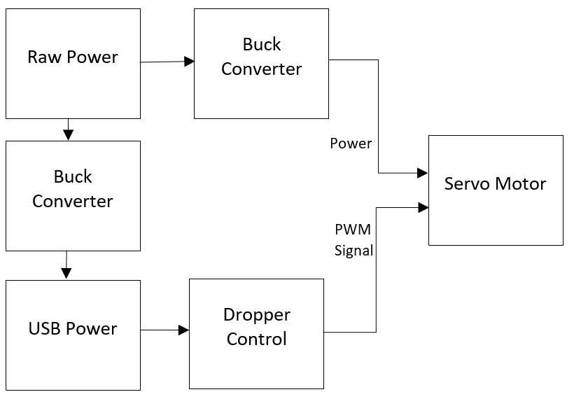
The dropper utilizes a servo motor and a DC-DC buck converter. Since the servo motor requires a larger current to operate correctly, a DC-DC buck converter was used to provide more current to the motor. The power line and ground were hooked up to the buck converter, and the dropper controller was connected to the signal line. The dropper controller utilizes an ATMEGA 1284P microcontroller. The microcontroller is powered over USB and operates at 3.3 volts. The signal line for the servo motor is hooked up to a PWM capable pin on the microcontroller. The code for the microcontroller utilizes the built-in PWM hardware for simplicity in the firmware. The firmware holds the servo in a certain position and regularly checks the UART for the value that tells the firmware to drop the payload in the dropper.

The last two tasks of the Robosub competition each year can be located by acoustic pingers which are setup near them. Locating the tasks by using these pingers requires a sonar system capable of determining the direction that a ping is coming from. Our sonar system accomplishes this by finding the time delays of the ping’s arrival at 4 hydrophones.

Our hydrophones

To get the time delays from the hydrophones, we first wait until the sound level reaches some threshold which indicates we are hearing a ping. We then perform cross correlations between the signal on channel 0 and the signals on the other channels. We shift the signal of each channel other than 0 over by a small amount of time and take the cross correlations between channel 0 again. This is repeated several times and then we take the shift value (a unit of time) of the max cross correlation for each channel as the time delay on that axis.

Cross correlating two sine functions at different offsets.

Once the time delays have been found, we can use trigonometry to determine what direction the sound came from. The image below shows how this is done in 2 dimensions, but the same idea applies to 3 dimensions.

Finding the ping angle from the time delays. Each dot labeled with an H represents a hydrophone. The red lines represent a sound wave at different times. The blue arrow represents the direction the sound came from.

Notice in the image that the angle θ is part of a right triangle. The hypotenuse of this triangle is the distance from one hydrophone to the other, and one side length is the time delay between those hydrophones multiplied by the speed of sound. Thus θ, which is the direction of the ping, can be found by taking the arccosine of that side length over the hypotenuse. Note that there are multiple angles which can have this cosine so we must also calculate the angle 90 – θ using the same method but with the other hydrophone (Hy). Knowing both θ and 90 – θ tells us what angle the ping came from so we can now use that information to navigate to the tasks.

Introduction

Over the last few months, James Irwin and I (Ryan Summers) have been working on a pretty fascinating engineering project for the Palouse Robosub club, and I figured I would give a quick write up on it. I want to put a forewarning here that I am a computer engineer, and some of the language below may be a bit technical, but I’m putting an effort into keeping the jargon to a minimum. 

In the competition, a major task (which awards quite a few points) involves a little bit of underwater acoustics. There’s a pinger somewhere in the pool that sends out pulses of sound every two seconds at anywhere from 25KHz – 40KHz. Through some clever triangulation algorithms (that are described here) and four different underwater microphones (from now on, I’m going to be calling these hydrophones), we have figured out that we can derive our position with respect to the pinger source by utilizing the depth of the pinger and of the submarine. It turns out the only pieces of information that we need is the different arrival times of the ping at four different hydrophones arranged in a specific configuration. Sounds easy right? It turns out it’s a bit more complicated than it first appears.

To set the stage for the difficulty of this project, we’ve had a variety of teams attempt to create a solution for the last four years, but none of them have been able to successfully deliver. These teams weren’t amateur engineers either – they were all full-fledged senior design teams. I even personally tried to take on the project with a half-baked solution of using a bare-metal raspberry pi project last summer with some minor success, but ultimately I didn’t finish in time for the competition. We’ve had a variety of ideas over the years and all of the different designs have helped to reform and refine our plans. This project has definitely taken both James and I out of our comfort zones, but I’m happy to see that it’s paying off so far.

An example of a cross-correlation. Taken from Giphy.

It turns out that the only way to effectively detect the ping (that we’ve been able to figure out so far, at least), is to continuously sample all of the hydrophones and perform a cross correlation (this means we basically slide signals across each other until they both overlap). Because of the sensitivity of our algorithm, we need to be able to tell the arrival times of the signal to within at least 1 microsecond, and the result needs to be fairly accurate. Otherwise, false positives can give us wildly different answers across different pings.

This effectively forms the basis of the problem. We have four hydrophones that we need to sample at a minimum rate of 1MHz each. Then, we need to correlate each of the signals to figure out the arrival time delays. Only then can we pass along that information to calculate our position. The hardware for sampling the hydrophones turned out to be more complicated than either me or James realized.

Hardware Selection

James and I had been eyeing the Zynq as a processor for this project. If you haven’t had the opportunity to work with the Zynq before, I would highly recommend it. It’s an extremely powerful device with a lot of potential for pretty much any project you throw at it. The Zynq 7010 boasts a dual ARM Cortex A9 processor suspended in FPGA fabric. Essentially, it’s a powerful computer surrounded by custom programmable digital logic. This means that you get the best of both worlds in terms of programmable logic and raw processing power because the processor can interact with the FPGA fabric as needed. We ended up selecting the LTC2171-14 as our ADC, as it could provide us simultaneous sampling on 4 channels from 5MHz - 65MHz, which was much higher than our initial requirement (go big or go home!).

We went looking around for Zynq development boards and came across the MicroZed. It was a pretty cool board that boasted expansion headers and differential trace routing. This meant that we could design our own circuit board to plug into the MicroZed and make sure to keep the differential traces safe. As a result of using the Zynq processor, the project has been dubbed the HydroZynq.

The layouts of revisions A through C are shown as the board gained complexity and decreased in size. 

Now that we had our hardware selected, we moved on to figured out exactly how any of this was going to work. Neither James or I knew anything about how the Zynq worked, so we had a lot to talk about for the next few days.

Implementation 

The custom circuit board was the first thing on our to-do list. Board printing usually takes about a month until you have a board sitting in your hand, and it rarely works the first time. We wanted to give ourselves plenty of time to figure out all of the bugs to make sure the hardware worked properly. The hydrophones we were using were the AS-1 from Aquarian Audio (shout out to Aquarian – they were absolutely wonderful to work with and the hydrophones we purchased from them are top-of-the-line). After about two weeks, I had made the schematic and laid out the board. More details about the specific implementation of the HydroZynq are available on our Wiki.

 The first revision of the HydroZynq board with the MicroZed mounted to it. 

Testing

The PCB came back as expected and I got to soldering it all together and made a fairly neat timelapse of the project. However, I realized halfway through soldering together the board that I had mirrored the two main MicroZed connectors. As a result, I had to do a lot of cut-and-jumpering to the board, but I’m happy to say that we managed to make the hardware work. Additionally, we found out that the FPGA I/O banks needed to be powered with 2.5V to utilize differential signaling. We had to cut out 1.8V power to it and supply an external 2.5V for testing.

A timelapse of soldering together the first version of the HydroZynq.

After soldering the board together, I got to testing it. Thankfully, there were some invaluable tools in debugging the hardware, FPGA, and software. The ADC chip has some options to output constant configurable data as opposed to the analog samples for testing. This means that you can tell it to give you a specific bit pattern, and each sample will be reported as that. This helps to verify the communication channel between the ADC and the FPGA. Additionally, Xilinx developed a tool called the Integrated Logic Analyzer (ILA). This allows you to record and probe different signals within the FPGA in real time. This was invaluable in debugging the hardware because I could look at exactly what the inputs to the FPGA were with nanosecond precision. It was this tool that was able to show me that a few of the pins on the ADC and connector weren’t quite soldered and didn’t have good contact.

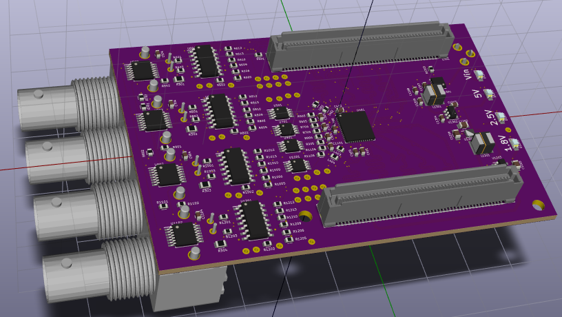
The second revision of the HydroZynq is smaller and more powerful (and less buggy). 

After initial testing, the bugs that we found were corrected and we developed a second revision of the board that was slightly smaller and easier to work with. We sent it out to the fabricator as we continued testing on the first revision.I made a timelapse of the creation of the board, but much of the internal routing footage got lost due to my screen recorder dying on me.

Timelapse of routing the HydroZynq for Rev B. 

 Construction of the HydroZynq's second revision. 

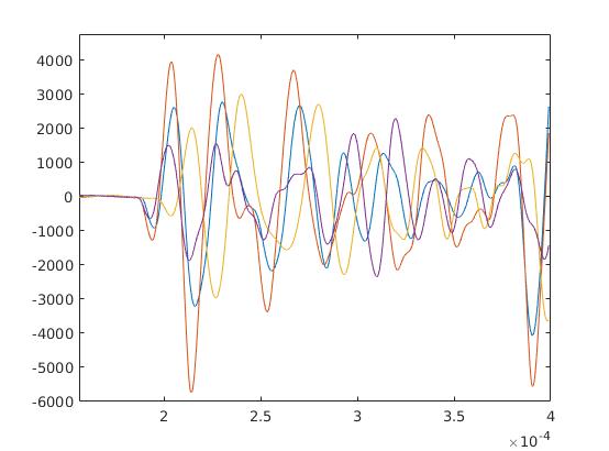
After getting all of the hardware functional, software development and debugging moved on.We made a second revision of the board and continued debugging the software. Once the new board came in, we put it together and started testing in a real pool environment with actual pings.

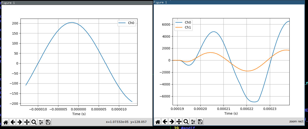
Ping data from testing in the pool was looking good!

After verifying some test signals, James and I moved on to testing the hardware with all of the hydrophones. After a bit of tinkering, we managed to convert the calculated arrival time delays into an angle of approach from the pinger. As we rotated the array and changed the heading towards the pinger, the hydrophone system correctly calculated the new angles.

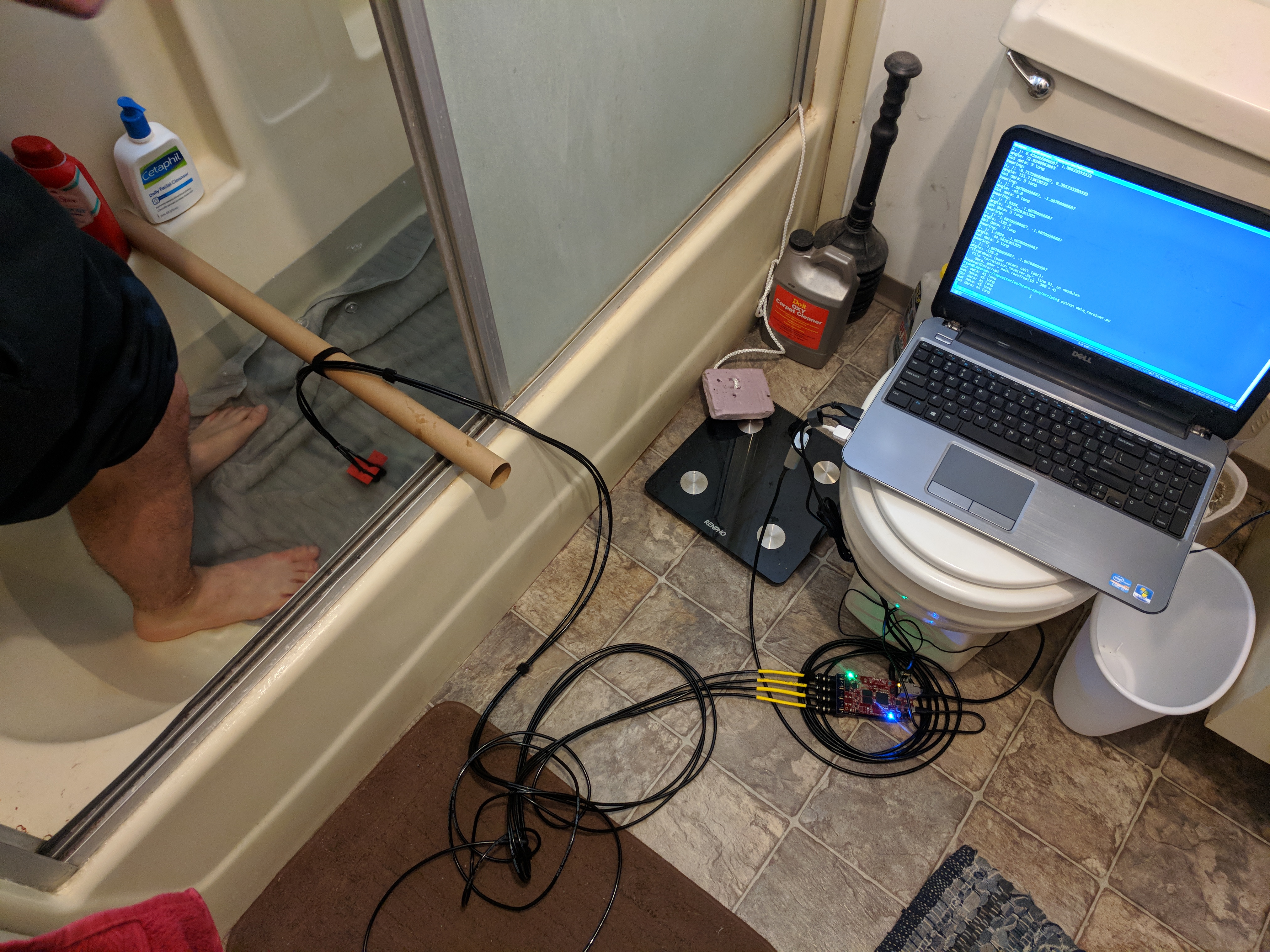
James and I had to rig up the system to test in the bathroom. 

The correlations and data started to look pretty good.

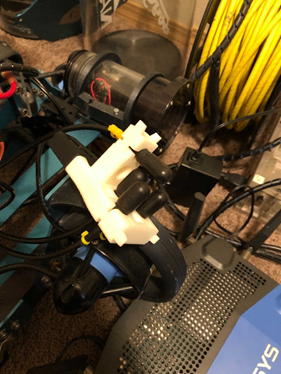
After verifying the functionality in the bathroom for the second board revision and a few tests in an actual pool with four hydrophones, we mounted the system onto the submarine for testing.

The 4 hydrophone phase array mounted on Cobalt,

We've done some initial testing with Cobalt and were able to get headings to the pinger from all the way across the pool! We're going to be testing an AI that goes to the pinger next weekend and I'll try to post an update about how it does.

The HydroZynq kit hooked up to cobalt and broadcasting data. 

We already have some changes for the final version of the board, and I'm sending out the design for printing soon.

The final revision of the HydroZynq has some additional features built into it for digitally adjustable gain.