While the Kalman Filter is simple and elegant, it is not always obvious what it is doing conceptually or mathematically. Constructing your own with a guide, or using a code package with instructions is quite possible to do without understanding the filter. However, when choices must be made about the code, the hardware, or the values, or when general problems arise, a more thorough understanding becomes paramount.

The true algorithm for the Kalman filter is covered in the Kalman Filter section. This introduction will instead incrementally construct an equivalent algorithm starting from the concept of simple Linear Least Square Estimation, using only basic matrix operations and basic statistics.

The Kalman Filter relies on a simple underlying concept – the linear least squares estimation. Given multiple noisy measurements of some state (speed, depth, acceleration, voltage, etc) the LLSE is an estimate that optimizes for the minimum of the sum of the squares of the errors.

In more formal terms, for some $m$ measurements $Y$ that are linear functions of a system with $n$ unknown states $X$ where $m>=n$. Such systems are said to be over-determined, whereby it is impossible to choose values of $X$ that will satisfy every measurement perfectly, and thus a compromise of values of $X$ is chosen that minimizes the total sum of the squares of the error between each measurement

$$ X_{est} = \text{arg}\,\min\limits_{\beta}\sum\|y-X\beta||^2 $$

Given the matrix format:

$$ \beta X = Y $$

$$ \begin{equation} \label{eq:control:expanded} \begin{bmatrix} \beta_{1,1} & \beta_{1,2} & \dots & \beta_{1,n} \\ \beta_{2,1} & \beta_{2,2} & \dots & \beta_{1,n} \\ \vdots & \vdots & \ddots & \vdots \\ \beta_{m,1} & \beta_{m,2} & \dots & \beta_{m,n} \end{bmatrix} \begin{bmatrix} X_{1} \\ X_{2} \\ \vdots \\ X_{n} \end{bmatrix} = \begin{bmatrix} Y_{1} \\ Y_{2} \\ \vdots \\ Y_{m} \\ \end{bmatrix} \end{equation} $$ This calculation could be performed iteratively, and the minimizing $X_{est}$ discovered, but with the measurements enumerated in this format, matrix arithmetic offers us a simple way to solve for $X_{est}$. For those that recall their Geometry class in high school, to solve for $X$ we need simply invert $\beta$ and multiply that inverse by both sides.

$$ \beta^{-1} \beta X = \beta^{-1} Y \\ IX = \beta^{-1} Y \\ X = \beta^{-1} Y $$

However, you can only invert square matrices. For all $m \neq n$ this won't be the case. Here we employ the Moore-Penrose LLSE calculation.

First both sides are multiplied by the transpose of $\beta$.

$$\beta' \beta X = \beta' Y $$

Recall: $$ \beta' = \begin{bmatrix} \beta_{1,1} & \beta_{2,1} & \dots & \beta_{m,1} \\ \beta_{1,2} & \beta_{2,2} & \dots & \beta_{n,1} \\ \vdots & \vdots & \ddots & \vdots \\ \beta_{1,n} & \beta_{2,n} & \dots & \beta_{n,m} \end{bmatrix} $$

$\beta' \beta$ will be a square matrix of size $n$. Assuming that at least one measurement of all states $X$ have been included, and indicated in $\beta$ this new square matrix will be invertable. We can then multiply both sides by that inverse to isolate the $X$ state vector.

$$ (\beta' \beta)^{-1}\beta' \beta X = (\beta' \beta)^{-1}\beta' Y \\ X = (\beta' \beta)^{-1}\beta' Y $$

Remarkably, this equation will give us an $X$ vector that satisfies the LLSE optimization.

If we want to fit a line to two points, both data points must satisfy the line equation $y = mx + b$.

$$y_1 = mx_1 + b, \\ y_2 = mx_2+b $$

We can pose the mathematical question in a matrix-format:

$$ \begin{bmatrix} x_1 & 1 \\ x_2 & 1 \end{bmatrix} \begin{bmatrix} m \\ b \end{bmatrix} = \begin{bmatrix} y_1 \\ y_2 \end{bmatrix} $$

Here our unknown slope and y-intercept $m$ and $b$ form our unknown state vector $X$. Our dependent measurements $y$ are used to construct our measurement vector $Y$, and the linear combination of independent variables and constants that relate that measurement to our state form $\beta$.

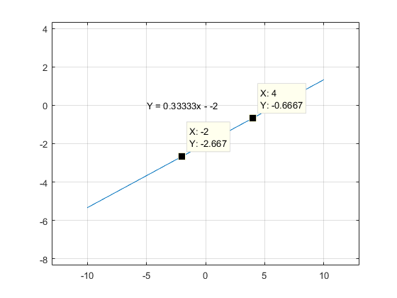
Given the two coordinate pairs $(-2, -\frac{8}{3})$ and $(4, -\frac{2}{3})$ we can find the line that is defined by them.

$$ \beta = \begin{bmatrix} -2 & 1 \\ 4 & 1 \end{bmatrix},\qquad X = \begin{bmatrix} m \\ b \end{bmatrix},\qquad Y = \begin{bmatrix} -\frac{8}{3} \\ -\frac{2}{3} \end{bmatrix} \\ \beta^{-1}Y = X \\ \begin{bmatrix} -2 & 1 \\ 4 & 1 \end{bmatrix}^{-1} \begin{bmatrix} -\frac{8}{3} \\ -\frac{2}{3} \end{bmatrix} = \begin{bmatrix} \frac{1}{3} \\ -2 \end{bmatrix} $$

Thus our slope $m = \frac{1}{3}$ and our linear offset $b = -2$.

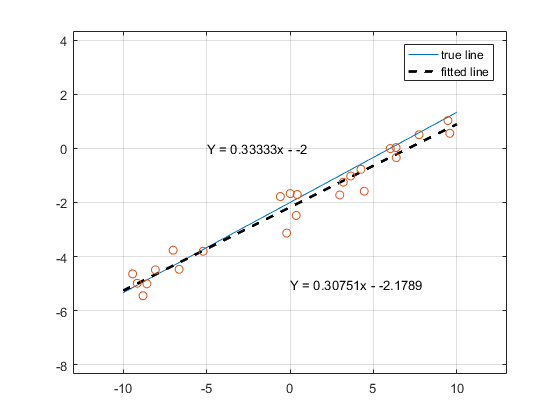
Now let's try fitting a line to an over-determined set of points. Below 20 points have been randomly generated. The x components were are uniformly random samples across domain $[-10, 10]$. The corresponding y components were first calculated directly using the true line equation $y = -\frac{1}{3}x -2$, and subsequently adding samples from a Gaussian random distribution with standard deviation $\sigma = 0.5$ .

$$ \beta = \begin{bmatrix} x_1 & 1 \\ x_2 & 1 \\ \vdots & \vdots \\ x_{20} & 1 \end{bmatrix}, \qquad X = \begin{bmatrix} m \\ b \end{bmatrix}, \qquad Y = \begin{bmatrix} y_1 \\ y_2 \\ \vdots \\ y_{20} \end{bmatrix} $$

We've just estimated our state based off of noisy measurements in an optimal fashion. At it's core, line-fitting like this is all that the Kalman Filter is doing. These next sections we will continuously build upon this basic function until we have something resembling the Kalman Filter.

We can guess intuitively that the noisier our sensors, the worse our estimation. Likewise, the more sensors (measurements) we obtain, the better our estimation. But exactly how much worse and how much better?

Let's consider 4 depth sensors. Each depth sensor makes a noisy measurement $z_n$ of the depth of our submarine.

For a quick refresher, a Guassian Random Variable has a 68% chance of falling within $\pm1\sigma$ and a 95% chance of falling within $\pm2\sigma$. The Variance (var)of the distribution is equal to $\sigma^2$. Standard Deviation (std) and var are interchangeable, and their usage depends mostly on ease of understanding, or ease of mathematical operations.

If we simply read of one depth sensor, the estimate of our depth will have an equal noise.

If we average the results of all four depth sensors, we will get a better estimate. Specifically, the Variance of an estimate is inversely proportional to the number of measurements $n$ taken.

$$z_1 \sim\mathcal{N}(0,\sigma^2),\qquad \frac{z_1 + z_2 + z_3 + z_4}{4} \sim\mathcal{N}(0,\frac{\sigma^2}{4}),\qquad $$

and thus the estimate from $n$ depth sensors of std $\sigma$ will have an std of $\frac{\sigma}{\sqrt{n}}$. For this example, we'll assume the noise is Gaussian, with a mean of zero (no bias) and a standard deviation of $\sigma = 2cm = 0.02m$. Thus, we'd expect the distribution of our estimate to be $\sigma/2$ or $0.01m$. Let's see if that happens.

$$ \beta = \begin{bmatrix} 1 \\ 1 \\ 1 \\ 1 \end{bmatrix},\qquad X = \begin{bmatrix}Z\end{bmatrix},\qquad Y = \begin{bmatrix} z_1 \\ z_2 \\ z_3 \\ z_4 \end{bmatrix} $$