While the Kalman Filter is simple and elegant, it is not always obvious what it is doing conceptually or mathematically. Constructing your own with a guide, or using a code package with instructions is quite possible to do without understanding the filter. However, when choices must be made about the code, the hardware, or the values, or when general problems arise, a more thorough understanding becomes paramount.

The true algorithm for the Kalman filter is covered in the Kalman Filter section. This introduction will instead incrementally construct an equivalent algorithm starting from the concept of simple Linear Least Square Estimation, using only basic matrix operations and basic statistics.

The Kalman Filter relies on a simple underlying concept – the linear least squares estimation. Given multiple noisy measurements of some state (speed, depth, acceleration, voltage, etc) the LLSE is an estimate that optimizes for the minimum of the sum of the squares of the errors.

In more formal terms, for some $m$ measurements $Y$ that are linear functions of a system with $n$ unknown states $X$ where $m>=n$. Such systems are said to be over-determined, whereby it is impossible to choose values of $X$ that will satisfy every measurement perfectly, and thus a compromise of values of $X$ is chosen that minimizes the total sum of the squares of the error between each measurement

$$ X_{est} = \text{arg}\,\min\limits_{\beta}\sum\|y-X\beta||^2 $$

Given the matrix format:

$$ \beta X = Y $$

$$ \begin{equation} \label{eq:control:expanded} \begin{bmatrix} \beta_{1,1} & \beta_{1,2} & \dots & \beta_{1,n} \\ \beta_{2,1} & \beta_{2,2} & \dots & \beta_{1,n} \\ \vdots & \vdots & \ddots & \vdots \\ \beta_{m,1} & \beta_{m,2} & \dots & \beta_{m,n} \end{bmatrix} \begin{bmatrix} X_{1} \\ X_{2} \\ \vdots \\ X_{n} \end{bmatrix} = \begin{bmatrix} Y_{1} \\ Y_{2} \\ \vdots \\ Y_{m} \\ \end{bmatrix} \end{equation} $$ This calculation could be performed iteratively, and the minimizing $X_{est}$ discovered, but with the measurements enumerated in this format, matrix arithmetic offers us a simple way to solve for $X_{est}$. For those that recall their Geometry class in high school, to solve for $X$ we need simply invert $\beta$ and multiply that inverse by both sides.

$$ \beta^{-1} \beta X = \beta^{-1} Y \\ IX = \beta^{-1} Y \\ X = \beta^{-1} Y $$

However, you can only invert square matrices. For all $m \neq n$ this won't be the case. Here we employ the Moore-Penrose LLSE calculation.

First both sides are multiplied by the transpose of $\beta$.

$$\beta' \beta X = \beta' Y $$

Recall: $$ \beta' = \begin{bmatrix} \beta_{1,1} & \beta_{2,1} & \dots & \beta_{m,1} \\ \beta_{1,2} & \beta_{2,2} & \dots & \beta_{n,1} \\ \vdots & \vdots & \ddots & \vdots \\ \beta_{1,n} & \beta_{2,n} & \dots & \beta_{n,m} \end{bmatrix} $$

$\beta' \beta$ will be a square matrix of size $n$. Assuming that at least one measurement of all states $X$ have been included, and indicated in $\beta$ this new square matrix will be invertable. We can then multiply both sides by that inverse to isolate the $X$ state vector.

$$ (\beta' \beta)^{-1}\beta' \beta X = (\beta' \beta)^{-1}\beta' Y \\ X = (\beta' \beta)^{-1}\beta' Y $$

Remarkably, this equation will give us an $X$ vector that satisfies the LLSE optimization.

If we want to fit a line to two points, both data points must satisfy the line equation $y = mx + b$.

$$y_1 = mx_1 + b, \\ y_2 = mx_2+b $$

We can pose the mathematical question in a matrix-format:

$$ \begin{bmatrix} x_1 & 1 \\ x_2 & 1 \end{bmatrix} \begin{bmatrix} m \\ b \end{bmatrix} = \begin{bmatrix} y_1 \\ y_2 \end{bmatrix} $$

Here our unknown slope and y-intercept $m$ and $b$ form our unknown state vector $X$. Our dependent measurements $y$ are used to construct our measurement vector $Y$, and the linear combination of independent variables and constants that relate that measurement to our state form $\beta$.

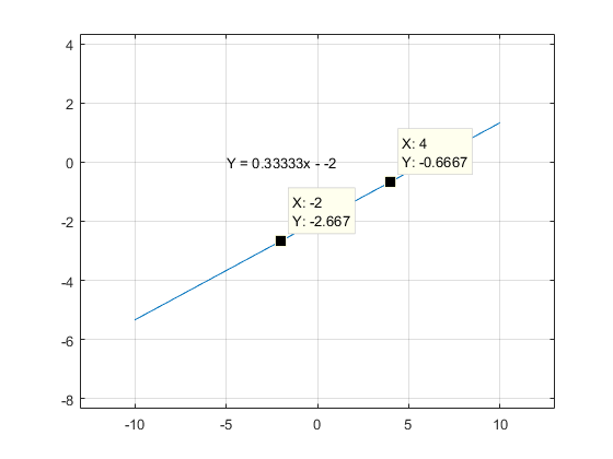
Given the two coordinate pairs $(-2, -\frac{8}{3})$ and $(4, -\frac{2}{3})$ we can find the line that is defined by them.

$$ \beta = \begin{bmatrix} -2 & 1 \\ 4 & 1 \end{bmatrix},\qquad X = \begin{bmatrix} m \\ b \end{bmatrix},\qquad Y = \begin{bmatrix} -\frac{8}{3} \\ -\frac{2}{3} \end{bmatrix} \\ \beta^{-1}Y = X \\ \begin{bmatrix} -2 & 1 \\ 4 & 1 \end{bmatrix}^{-1} \begin{bmatrix} -\frac{8}{3} \\ -\frac{2}{3} \end{bmatrix} = \begin{bmatrix} \frac{1}{3} \\ -2 \end{bmatrix} $$

Thus our slope $m = \frac{1}{3}$ and our linear offset $b = -2$.

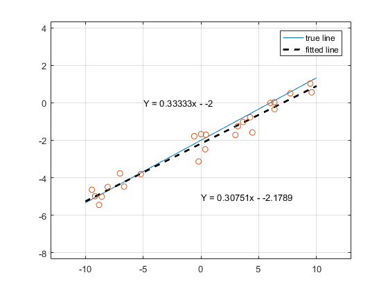
Now let's try fitting a line to an over-determined set of points. Below 20 points have been randomly generated. The x components were are uniformly random samples across domain $[-10, 10]$. The corresponding y components were first calculated directly using the true line equation $y = -\frac{1}{3}x -2$, and subsequently adding samples from a Gaussian random distribution with standard deviation $\sigma = 0.5$ .

$$ \beta = \begin{bmatrix} x_1 & 1 \\ x_2 & 1 \\ \vdots & \vdots \\ x_{20} & 1 \end{bmatrix}, \qquad X = \begin{bmatrix} m \\ b \end{bmatrix}, \qquad Y = \begin{bmatrix} y_1 \\ y_2 \\ \vdots \\ y_{20} \end{bmatrix} $$

We've just estimated our state based off of noisy measurements in an optimal fashion. At it's core, line-fitting like this is all that the Kalman Filter is doing. These next sections we will continuously build upon this basic function until we have something resembling the Kalman Filter.

We can guess intuitively that the noisier our sensors, the worse our estimation. Likewise, the more sensors (measurements) we obtain, the better our estimation. Bayesian statistics tells us that all information, no matter how noisy, is still good information. Indeed the entire point of this field of mathematics is to get very accurate estimations from a combination of far-less accurate measurements. But exactly how much better do our estimates get?

Let's consider 4 depth sensors. Each depth sensor makes a noisy measurement $z_n$ of the depth of our submarine.

For a quick refresher, a Guassian Random Variable has a mean and a variance. The Variance (var)of the distribution is equal to $\sigma^2$. Standard Deviation (std) is simply $\sigma$. Std and var are both perfectly valid ways to describe the distribution, and their usage depends mostly on ease of understanding, or ease of mathematical operations. As a good way to conceptualize what the std translates to, 68% of values pulled from a Gaussian distribution will be within $\pm1\sigma$ of the mean. 95% of the values will fall within $\pm2\sigma$.

If we simply read of one depth sensor, the estimate of our depth will have an equal noise.

If we average the results of all four depth sensors, we will get a better estimate. Specifically, the Variance of an estimate is inversely proportional to the number of measurements $n$ taken.

$$z_1 \sim\mathcal{N}(0,\sigma^2),\qquad \frac{z_1 + z_2 + z_3 + z_4}{4} \sim\mathcal{N}(0,\frac{\sigma^2}{4}),\qquad $$

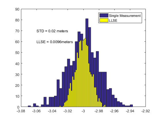
and thus the estimate from $n$ depth sensors of std $\sigma$ will have an std of $\frac{\sigma}{\sqrt{n}}$. For this example, we'll assume the noise is Gaussian, with a mean of zero (no bias) and a standard deviation of $\sigma = 2cm = 0.02m$. The actual depth we're measuring is $3m$ Thus, we'd expect the distribution of our estimate to be $\sigma/2$ or $0.01m$. Let's see if that happens.

$$ \beta = \begin{bmatrix} 1 \\ 1 \\ 1 \\ 1 \end{bmatrix},\qquad X = \begin{bmatrix}Z\end{bmatrix},\qquad Y = \begin{bmatrix} z_1 \\ z_2 \\ z_3 \\ z_4 \end{bmatrix} \\ X_{est} = (\beta'\beta)^{-1}\beta Y $$

If we create a script that generates 4 measurements by taking our true depth and adding a sample from a Guassian distribution with std $\sigma = 0.02$, then we can use the above equation to estimate our depth. $y_{1,2,3,4} = 3 + \sim\mathcal{N}(0,.02^2)$. If we estimate our depth 1000 times, we should get a distribution of estimated depths that has a standard deviation of $\frac{\sigma}{\sqrt{4}} = \frac{0.02m}{2} = 0.01m$.$

Now we know how confident we can be in our estimates given multiple, identical sensors.

The underlying assumption of the Linear Least Squares Estimation is that all measurements hold equal weight. That is to say, all are equally noisy and should be trusted equally. This can work well for fusing the results of duplicate sensors, but becomes a poor assumption when combining different sensors.

Some of the cleverer readers might be thinking of a simple workaround – just add copies of the more accurate sensors' measurements into the matrix so the system listens to them more. And that’d certainly emulate what we’re trying to do. But it’s not mathematically perfect, nor is it elegant to code or computationally efficient to run.

If you have different sensors of different quality, we need to move to the Weighted Linear Least Squares Estimation (WLLSE).

Before for LLSE we had:

$$ X = (\beta' \beta)^{-1}\beta' Y $$

Our new equation for *WLLSE* is:

$$ X = (\beta'W \beta)^{-1}\beta' WY,\qquad W = \begin{bmatrix} \frac{1}{\sigma_{1}^2} & 0 & \dots & 0 \\ 0 & \frac{1}{\sigma_{2}^2} & \dots & 0 \\ \vdots & \vdots & \ddots & \vdots & \\ 0 & 0 & \dots & \frac{1}{\sigma_{n}^2} \end{bmatrix} $$

Working out the exact operations going on here is an exercise left to the student. However, intuitively we can see what's happening. When you multiply a matrix by an identity matrix $I_n$ it remains unchanged. More generally, If you multiply a matrix by a diagonal matrix, it will scale each row or column (depending on order of operation) by it's corresponding value. Here we're inserting a scaling diagonal matrix in the middle of our LLSE solution. And we're scaling each value by the inverse of its variance.

Thus, measurements enumerated in the $\beta$ matrix with low variances will be scaled by large numbers, and those with large variances will be similarly shrunk. In this way, the measurements are given more weight according to how well they can be trusted.

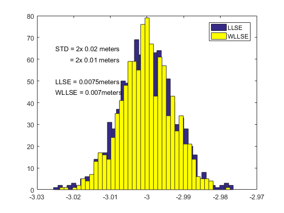
If we repeat our example from Section 1.2, but reduce the noise of two of the depth sensors, we should get an ever better estimation. For Depth sensors 1 and 2, $\sigma = 0.02m$. For Depth Sensors 3 and 4, $\sigma = 0.01$.

$$ \beta = \begin{bmatrix} 1 \\ 1 \\ 1 \\ 1 \end{bmatrix},\qquad X = \begin{bmatrix}Z\end{bmatrix},\qquad Y = \begin{bmatrix} z_1 \\ z_2 \\ z_3 \\ z_4 \end{bmatrix},\qquad W = \begin{bmatrix} \frac{1}{0.02^2} & 0 & 0 & 0 \\ 0 & \frac{1}{0.02^2} & 0 & 0 \\ 0 & 0 & \frac{1}{0.01^2} & 0 \\ 0 & 0 & 0 & \frac{1}{0.01^2} \end{bmatrix} \\ X_{est} = (\beta'W\beta)^{-1}\beta WY $$

Recall that in Section 1.2 we used four depth sensors of std $\sigma_z = 0.02$ and got an estimate with std $\sigma_{est} = 0.01m$.

By using a regular LLSE, where we assume all four depth sensors are equally trustworthy, we get a reduced std of $\sigma_{est} = 0.0075m$ simply by virtue of having more accuracy in some sensors. However, by using WLLSE we tighten the estimate down to $\sigma_{est} = 0.007$. Both estimates made here were made with identical information. The only question was how we processed that information. In this regard, appropriately trusting different sensors by different amounts gives us an overall better estimate.

However, the question now is, exactly how much should we trust our overall estimate? It's fine to make many estimates many times and find that distribution, but there should be some way to mathematically know how trustworthy our estimate is, based off of how trustworthy our various sensors were.

There is. In fact, we already calculated it. $$ R = inv(\beta' W \beta) = 5.413e^{-5},\qquad R = \begin{bmatrix} \sigma_{1}^2 & \sigma_{1}\sigma_{2} & \dots & \sigma_{1}\sigma_{n} \\ \sigma_{2}\sigma_{1} & \sigma_{2}^2 & \dots & \sigma_{2}\sigma_{n} \\ \vdots & \vdots & \ddots & \vdots & \\ \sigma_{n}\sigma_{1} & \sigma_{n}\sigma_{2} & \dots & \sigma_{n}^2 \end{bmatrix} \\ \sigma^2 = 5.413e^{-5},\qquad \sigma = 0.0756 $$

Where R is the co-variance matrix of the estimated state. The diagonals of R reflect the variance of each estimated state. The off-diagonal terms are co-variances. Put simply, two random variables can have normal distributions, but share some underlying property that makes them correlate. If one is above the mean, the other is likely above the mean. Or vice-versa. This is important when you start trying to calculate things from linear combinations of state elements. Mathematically, $$var(aX+bY) = a^2Var(X) + b^2Var(Y) + 2abCov(X,Y)$$. Normally separate states will be uncorrelated, and have $Cov(X,Y)=0$. However, when you're dealing with physical models and sensors, correlations start to pop up, like the position and the velocity of your vehicle.

If you had an overestimated position but an underestimated velocity, and you try to predict where you'll be in 1 second, your predicted position could be pretty accurate. But over time, if your velocity is being under-estimated for too long, you're also likely underestimating your position. If you know that more often that not, your position and velocity are both over or under estimated, it's more likely the predicted position based on your estimates is further from the true position than if they were uncorrelated.

Thus, if you try to predict your location 1 second in the future, $x[k+1] = x[k] + \dot{x}[k] * 1sec$, the variance of that predicted location isn't going to simply be the noise of your current position plus the noise of your velocity, but additionally some extra noise because both states are inter-related and more liable to compound their noise rather than counteract it. That's where the $2cov(X,Y)$ term comes in.

And if you think that equation for variance looks remarkably like the Law of Cosines in Trigonometry - Congratulations. You get a cookie.

Taking a break from probability and estimation, we need to consider how to model a system in time. Think of it like modeling the position of a shell fired from a cannon. Physics 101 stuff.

We’re going to put our system into something called the State-Space format. It equates the derivative of the system as a linear function of the current state of the system, plus any current external forces.

$$\dot{x}(t) = Ax(t) + Bu(t)$$

where $x(t)$ is the current state and $u(t)$ are inputs to the state. The reasons for putting it in this form are good, but can be a little unclear in the continuous time domain. Since the Kalman Filter operates in discrete-time anyway, we’ll move there. The equivalent form is:

$$x[k+1] = Ax[k] + Bu[k]$$

Where we model the next state as a linear function of our current state and current inputs. As an example, let’s say our state is a vector of two variables, a position vector $x$, and our velocity, $\dot{x}$, and we want to make a discrete-time model of our system with position, velocity, and acceleration. Our State Space representation would be:

$$ x[k+1] = x[k] + \dot{x}[k]dt + \frac{1}{2}\ddot{x}[k]dt^2 \\ \dot{x}[k+1] = \dot{x}[k] + \ddot{x}[k]dt \\ X = \begin{bmatrix} x \\ \dot{x} \end{bmatrix},\qquad A = \begin{bmatrix} 1 & dt \\ 0 & 1 \end{bmatrix},\qquad B = \begin{bmatrix} \frac{dt^2}{2} \\ dt \end{bmatrix},\qquad u = \ddot{x} $$

For computer modeling, you can see why this is a very useful format. Matrix $A$ called the Transition Matrix, multiplied by the current state $X$ will calculate the state $X$ at the next time-step, barring any inputs. External inputs influence the system through the $B$ matrix, appropriately called the Input Matrix.

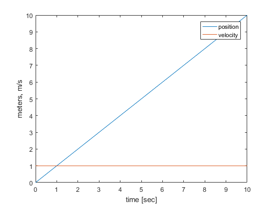
Simply placing this equation into a for loop will allow you to model the system iteratively. Here is a system with an initial position of $0m$ and an initial velocity of $1m/s$ with no external input.

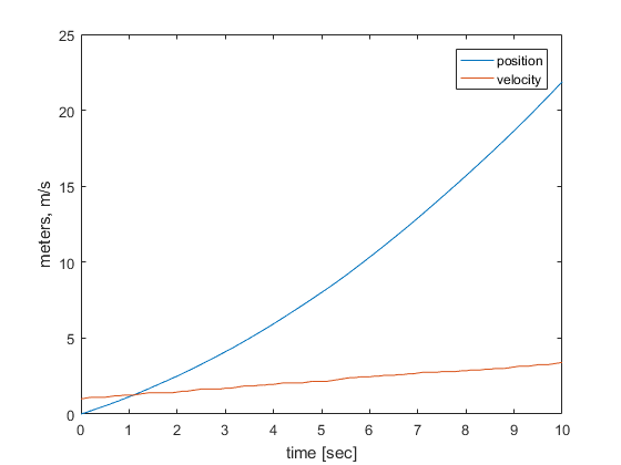
That's rather boring, however. Here's a more interesting version, with random inputs.

It doesn't look like much, but this format is infinitely scalable in complexity. Linear systems with two, or ten, or two hundred states can all have their dynamics modeled in this simple manner. But we'll leave building our Submarine model for a different tutorial.

The second part of the State Space format is the measurement vector equation.

$$ Y[k] = CX[k] + Du[k] $$

This model doesn't iterate the future, but rather calculates measurements $Y$ of sensors, as linear functions of the state $X$, specified by the Emission Matrix $C$. Matrix $D$ specifies distortions to measurements that occur as functions of the input. While inputs distorting sensors is not uncommon, matrix D is seldom used. Often distortions from inputs are removed from the measurements separately, as a form of calibration, prior to solving for state estimations.

In our previous examples with depth sensors, C was a simple vector of $1s$ because our only state was depth, and it was being measured directly. As with the Transition matrix, the Emission matrix can rapidly become complex as the type of sensors, states, and measurements being considered expand. However, creating the Emission Matrix will be covered under a different Localization Topic. Here, all we care about is creating a systematic format for our system dynamics and our sensor measurements.

Let's use our State Space Model to make an example with our Depth Sensors.

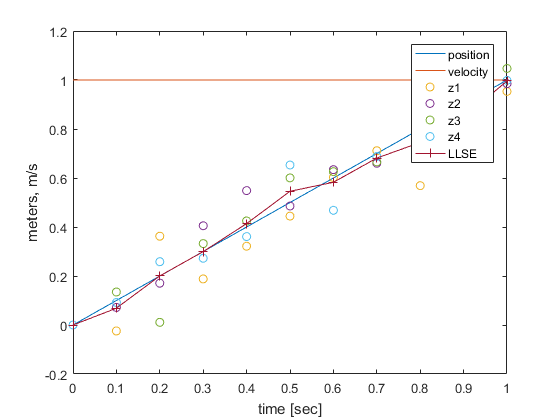
$$ dt = 0.1sec,\quad X[0] = \begin{bmatrix} 0m \\ 1ms^-1 \end{bmatrix},\quad u = 0,\quad A = \begin{bmatrix} 1 & 0.1 \\ 0 & 1 \end{bmatrix},\quad B = \begin{bmatrix} 0.005 \\ 0.1 \end{bmatrix},\quad C = \begin{bmatrix} 1 & 0\\ 1 & 0\\ 1 & 0\\ 1 & 0 \end{bmatrix},\quad $$ and we'll use our emission matrix to generate measurements $Y[k]$ from our true state $X[k]$, add noise of $\sigma = 0.08m$, and then calculate an estimate of our position $x_{est}[k]$ through our LLSE equation.

Modeling this from $t=[0,1]$ gives us:

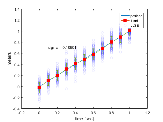
That seems to track the true state pretty well. Let's see exactly how well, by following the state 1000 times.

We see that at each point in time, we take many measurements, and estimate a position that is close to our true position. If we did this 1000 times, we can see how accurate we are at tracking our system at any one time. If you notice, our error in measurement at any point in time is roughly constant.

Next, we’ll see how we can do better.